Excel Cross Out Cell: Effective Formatting Techniques

To cross out a cell in Excel, select the cell(s) you want to format, then go to the “Format Cells” dialog box, and under the “Effects” tab, click on “Strikethrough.” This will apply the strikethrough formatting to the selected cell(s).
You can then save the workbook and reopen it to see the changes. Excel is a widely used spreadsheet program that offers various formatting options to enhance the appearance and readability of data. One such formatting option is the ability to cross out cells, which can be useful for indicating completed tasks or canceled items.
We will explore how to cross out a cell in Excel using the built-in strikethrough feature. By following a few simple steps, you can easily apply strikethrough formatting to cells and modify your data presentation in Excel. Let’s dive in and learn how to cross out a cell in Excel.
Exploring Different Methods
There are several ways to cross out a cell in Excel, each offering its own benefits and convenience. In this section, we will cover three main methods: adding a diagonal line, applying strikethrough, and using a shortcut for strikethrough.
Adding A Diagonal Line
One of the ways to cross out a cell in Excel is by adding a diagonal line. This method is useful when you want to visually indicate that the data in a cell is no longer valid or relevant. Here’s how you can do it:
- Click on the cell where you want to add the diagonal line.
- Go to the “Format” tab in the Excel ribbon.
- Click on the “Borders” button in the “Font” group.
- In the “Borders” dropdown menu, select “Diagonal Down” or “Diagonal Up” depending on how you want the line to appear.
- The diagonal line will now be added to the cell, crossing it out.
This method allows you to customize the appearance of the diagonal line, giving you more control over how it looks.
Applying Strikethrough
Another method to cross out a cell in Excel is by applying strikethrough. This method is quick and straightforward, making it ideal for simple tasks. Here’s how you can do it:
- Select the cell or cells that you want to cross out.
- Right-click on the selected cell(s) and choose “Format Cells” from the context menu.
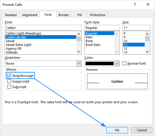
- In the “Format Cells” dialog box, go to the “Font” tab.
- Check the “Strikethrough” checkbox under the “Effects” section.
- Click “OK” to apply the strikethrough formatting.
This method is especially useful when you want a quick and easy way to visually indicate that a cell’s content is no longer valid.
Shortcut For Strikethrough
If you frequently use the strikethrough formatting in Excel, you might find it more efficient to use a keyboard shortcut. This method allows you to quickly cross out cells without having to navigate through menus. Here’s the shortcut you can use:
- Select the cell or cells that you want to cross out.
- Press the “Ctrl + 5” keys on your keyboard.
By using this shortcut, you can easily apply strikethrough formatting to cells in just a few keystrokes. It saves you time and allows for a more efficient workflow.

Credit: resume.io
Customization Options
When it comes to customizing your Excel spreadsheet, you’ll be happy to know that there are several options available to you. Among these options, you can easily cross out cells to signify completion, strike through data for deletion, or add hatching patterns to enhance the visual appeal of your spreadsheet. In this section, we’ll explore each of these customization options in detail.
Formatting Diagonal Lines
If you want to add a diagonal line to a cell in Excel, it’s a simple process that can be done in just a few clicks. To get started, follow these steps:
- Select the cell or range of cells where you want to add the diagonal line.
- Click on the “Format” tab in the Excel ribbon.
- In the “Format Cells” dialog box, go to the “Border” tab.
- Choose the layout for the diagonal line under the “Diagonal” section.
- Click “OK” to apply the formatting and see the diagonal line in your selected cell(s).
Changing Line Colors
To make your diagonal line stand out, you can also change its color to match your desired aesthetic. Here’s how you can change the color of the diagonal line:
- Select the cell(s) with the diagonal line.
- Go to the “Format” tab in the Excel ribbon.
- In the “Format Cells” dialog box, navigate to the “Border” tab.
- Click on the color palette icon next to the diagonal line options.
- Select your desired color from the palette or enter a custom RGB value.
- Click “OK” to apply the color change to your diagonal line.
Inserting Hatching Patterns
If you want to add some visual flair to your spreadsheet, inserting hatching patterns can be an excellent choice. Follow these steps to insert hatching patterns:
- Right-click on the shape or cell where you want to insert hatching patterns.
- Select “Format Shape” from the menu that appears.
- In the left pane of the “Format Shape” dialog box, click on “Fill”.
- In the right pane, select the “Pattern Fill” radio button.
- Choose from the various hatching pattern options available.
- Click the “Close” button to apply the hatching pattern to your shape or cell.
With these customization options at your disposal, you can easily enhance the presentation and readability of your Excel spreadsheets. Whether you need to cross out cells, change line colors, or insert hatching patterns, Excel gives you the tools to make your data stand out.
Utilizing Quick Access Features
Quick Access Features in Excel can significantly enhance your productivity by providing easy access to essential functions. One of the handy features is the ability to insert a strikethrough icon directly on your toolbar for quick formatting options.
Inserting Strikethrough Icon
Adding the strikethrough icon to your Quick Access Toolbar is a simple process that can save you time when formatting cells in Excel. Here’s how you can do it:
- Right-click on any existing QAT icon.
- Select “Customize Quick Access Toolbar.”
- Choose ‘All Commands’ from the dropdown list on the left.
- Scroll down and select the “Strikethrough” command.
- Click on “Add”.
Customizing Quick Access Toolbar
Customizing your Quick Access Toolbar in Excel allows you to tailor it to your specific needs, ensuring that essential functions are readily accessible. Here’s how you can customize your QAT:
- Right-click on any existing QAT icon.
- Select “Customize Quick Access Toolbar.”
- Choose ‘All Commands’ from the dropdown list on the left.
- Select the functions you frequently use and add them to the toolbar for easy access.
Recognizing Helpful Tools
If you are an Excel user, you may be familiar with the frustration of not being able to locate the right tool to help you with your tasks. Many times, you may have wondered if there are tools that could enhance your experience and make your work more efficient. Recognizing helpful tools is essential, and in the case of Excel, there are several options available that can significantly improve your productivity and workflow. Let’s explore some of these valuable tools that can make a real difference in your Excel experience.
Excel Powerups Premium Suite
Excel PowerUps Premium Suite offers a range of powerful tools designed to streamline your Excel workflow. From advanced formatting options to data analysis features, this suite provides a comprehensive set of tools to enhance your Excel experience. With a focus on efficiency and productivity, Excel PowerUps Premium Suite is a valuable addition to any Excel user’s toolkit.
Zebra Bi Integration
Zebra BI Integration is a game-changer for Excel users, offering advanced functionalities for data visualization and reporting. This integration brings a new level of sophistication to Excel, allowing users to create dynamic and visually appealing reports with ease. With its intuitive interface and powerful features, Zebra BI Integration is a must-have tool for anyone looking to elevate their Excel skills.
Goskills Assistance
GoSkills Assistance offers a range of resources and training materials to help Excel users improve their skills and master the intricacies of the software. Whether you are a beginner looking to learn the basics or an advanced user seeking to become a power user, GoSkills Assistance has something to offer for everyone. With its user-friendly interface and comprehensive learning materials, GoSkills Assistance is an invaluable resource for anyone looking to excel in Excel.
Mastering Shortcuts And Techniques
Applying Keyboard Shortcuts
Excel offers a plethora of shortcuts that expedite processes and save time. To apply strikethrough formatting, simply press Ctrl + 5 on your keyboard. Equally convenient is the Quick Access Toolbar, where you can add the Strikethrough command for easy access. Mastering these shortcuts improves efficiency and fluency in Excel usage.
Understanding Excel Borders
Excel’s formatting options go beyond basic cell content. Learning to insert hatching and customize borders elevates the visual presentation of your data. By right-clicking on shapes and utilizing the Format Shape menu, you can easily implement hatching patterns and border styles, enhancing the clarity and organization of your Excel spreadsheets.
Optimizing Formatting Methods
Leveraging the Strikethrough option in Excel is just one aspect of optimizing formatting methods. Additionally, users can access the Conditional Formatting Manager for advanced conditional formatting techniques. This feature enables customization and fine-tuning of formatting rules, providing a comprehensive toolset to elevate the visual appeal and clarity of Excel data.
Credit: www.ablebits.com

Credit: resume.io
Frequently Asked Questions Of Excel Cross Out Cell
Is There A Way To Cross Out A Cell In Excel?
To cross out a cell in Excel, select the desired cell, go to Format Cells > Effects > Strikethrough. Save and reopen for changes to appear.
What Is Shortcut For Strikethrough In Excel?
To apply strikethrough to a cell in Excel, you can use the shortcut Ctrl + 5. Simply select the cell(s) you want to strikethrough and press Ctrl + 5 on your keyboard. This will cross out the cell content.
How Do You Cross Hatch A Cell In Excel?
To cross hatch a cell in Excel, right-click the cell and select “Format Cells. ” Then, under the Fill tab, click the “Pattern Fill” radio button and choose a hatching pattern. Click “Close” to apply the hatch.
How Do I Insert A Strikethrough Icon In Excel?
To insert a strikethrough icon in Excel, click on any ribbon tab and select Customize the Ribbon. Choose ‘All Commands’ and add the Strikethrough command.
Conclusion
To effectively cross out a cell in Excel, simply follow the steps mentioned above. Utilize the Strikethrough option for easy formatting. Ensure to save and reopen for the changes to take effect. This straightforward method enhances data presentation and clarity in Excel spreadsheets.
Enhance your Excel skills today!