How to Unhide Rows in Google Sheets

To unhide rows in Google Sheets, select the rows directly above and below the hidden row, right-click, and choose “Unhide Rows.” When it comes to working with Google Sheets, hiding rows can sometimes make important data inaccessible.

If you’ve accidentally hidden rows and need to unhide them, the process is simple and straightforward. By selecting the rows directly adjacent to the hidden row, right-clicking, and choosing “Unhide Rows,” you can quickly restore visibility to all your hidden rows and access the data you need.

This guide will walk you through the steps to unhide rows in Google Sheets, ensuring that you can easily retrieve any rows that may have gone missing.

Table of Contents

Methods To Unhide Rows

To unhide rows in Google Sheets, there are different methods you can employ. Each method offers a simple way to reveal the hidden rows in your spreadsheet. Let’s explore the various methods to unhide rows:

Direct Unhiding

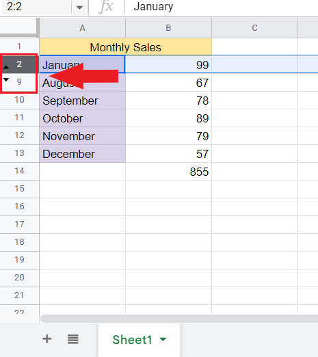
Select the rows directly above and below the hidden row.
Right-click with your mouse.
Click on “Unhide Rows” to make the hidden rows visible again.

Using Filters

Turn off any filters you may have applied to your data.
Click on the filter button in the spreadsheet toolbar to disable the filter views.
Check if your hidden rows reappear once the filters are turned off.

Credit: www.lifewire.com

Troubleshooting

Easily unhide rows in Google Sheets by selecting the rows above and below the hidden one, then right-click and choose “Unhide Rows. ” This simple step resolves any visibility issues and ensures all information is readily accessible within your spreadsheet.

Hidden Rows Not Visible

If your hidden rows are not visible in Google Sheets, there could be a few reasons for this issue.

Check if the rows are filtered or have any applied sorting. This may cause the hidden rows to be temporarily invisible.
To resolve this, go to the “Data” tab and click on “Filter” to see if any filters are applied. Clear any filters to display all rows.
Another possibility is that there might be a formatting issue with the rows. Make sure there are no formatting rules or conditional formatting applied that may hide the rows.
In such cases, select the hidden rows directly above and below the hidden ones. Right-click, and then click “Unhide Rows”. This should make the hidden rows visible again.

Arrows To Unhide Not Showing

If you are unable to see the arrows to unhide rows in Google Sheets, there are a few steps you can take to resolve this problem.

First, ensure that you have selected the correct rows. Verify that you have highlighted the rows directly above and below the hidden ones.
If the arrows still do not appear, it could be due to a display or browser issue. Try refreshing the page or using a different browser to see if the arrows reappear.
Alternatively, clearing your browser cache and cookies may also help resolve the issue.
If none of the above solutions work, try accessing Google Sheets in an incognito or private browsing mode, as this can sometimes bypass certain display issues.

Advanced Techniques

Unhiding rows in Google Sheets is a fundamental skill, but did you know that there are advanced techniques that can help you save time and work more efficiently? In this section, we will explore two powerful techniques – Freezing Rows and Keyboard Shortcuts.

Freezing Rows

Freezing rows can be incredibly useful when working with large datasets in Google Sheets. It allows you to keep certain rows visible at all times while scrolling through the rest of your sheet. Here’s how you can do it:

Select the row below which you want to freeze. This means that all rows above that selected row will remain visible.
Go to the top menu and click on View.
Hover over the Freeze option and select 1 Row or the number of rows you want to freeze.

Keyboard Shortcuts

If you’re someone who loves using keyboard shortcuts to speed up your workflow, Google Sheets has you covered. Here are some useful keyboard shortcuts to unhide rows:

Keyboard Shortcut	Action
Ctrl + Shift + 9	Unhide rows

Simply select the hidden rows, press Ctrl + Shift + 9, and watch them magically appear!

By utilizing these advanced techniques – Freezing Rows and Keyboard Shortcuts – you can enhance your productivity and make working with Google Sheets even easier. Try them out and see how they can simplify your workflow.

Credit: www.simplesheets.co

Frequently Asked Questions On How To Unhide Rows In Google Sheets

How Do I Unhide All Rows In Google Sheets?

To unhide all rows in Google Sheets, select the rows above and below the hidden ones, right-click, and choose “Unhide Rows. “

How Do I Unhide Hidden Rows?

To unhide hidden rows in Google Sheets, select the rows above and below the hidden ones, then right-click and choose “Unhide Rows. “

Why Are Rows Missing On My Google Sheet?

The rows may be hidden due to filters. Turn off the filters to reveal all rows.

How Do I Make Rows Always Visible In Google Sheets?

To make rows always visible in Google Sheets, you can freeze them. Open the spreadsheet, select the row or column you want to freeze, click “View” at the top, and then select “Freeze” to specify how many rows or columns you want to freeze.

Conclusion

To unhide rows in Google Sheets, simply select adjacent rows, right-click, and choose “Unhide Rows. ” The process is quick and straightforward. Remember to check for any filters that may be hiding your rows, and disable them to reveal all your data effortlessly.

Mastering this feature enhances your spreadsheet efficiency.