How to Strike Through Text in Excel

To strike through text in Excel, select the cell or range of cells, then go to the ‘Font’ section in the ‘Home’ tab, click on the ‘Format Cells’ dialog box launcher, and under the ‘Font’ tab, check the ‘Strikethrough’ box. Adding strikethrough in Excel is a simple process that enhances the presentation of your data.

It allows you to visually indicate that certain information is no longer valid or applicable, making it a useful tool for data management. Whether you are working on financial reports, inventory lists, or any other type of spreadsheet, applying a strikethrough effect can help convey changes or updates effectively.

By following a few simple steps, you can easily apply this formatting to your Excel sheets, making your data more visually appealing and easy to understand. Additionally, using keyboard shortcuts can streamline the process, providing a faster way to format your data.

Credit: www.ablebits.com

Table of Contents

Methods Of Applying Strikethrough In Excel

Strikethrough text is a formatting option in Excel that is commonly used to indicate deleted or irrelevant information. Applying strikethrough to text can be done using different methods, depending on your convenience and preference. In this article, we will explore two popular methods of applying strikethrough in Excel: using Ribbon/Menu options and utilizing keyboard shortcuts.

Using Ribbon/menu Options

If you prefer a graphical user interface, using the Ribbon or Menu options in Excel is a straightforward way to apply strikethrough to text. Follow these steps:

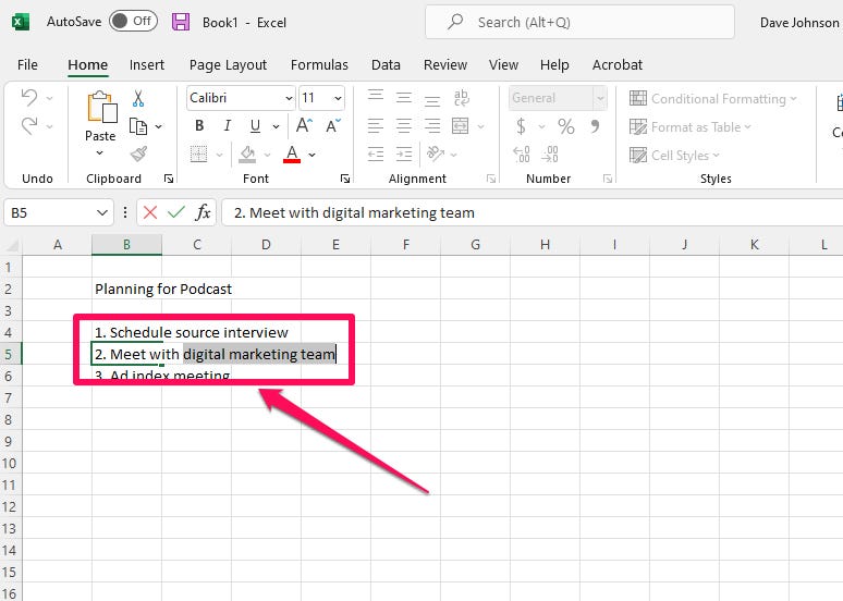
Select the cell(s) or text containing the information you want to strikethrough.
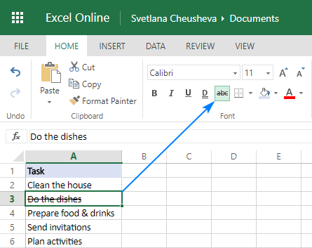
Go to the Home tab in the Excel Ribbon.
Locate the Font group, which contains various formatting options.
Click on the small arrow at the bottom-right corner of the Font group.
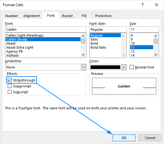
In the Format Cells dialog box that appears, navigate to the Font tab.
Check the box next to Strikethrough under the Effects section.
Click OK to apply the strikethrough formatting to the selected text.

Utilizing Keyboard Shortcuts

For those who prefer a quicker and more efficient method, utilizing keyboard shortcuts in Excel is the way to go. Here’s how you can apply strikethrough using keyboard shortcuts:

Select the cell(s) or text you want to strikethrough.
Press Ctrl + 5 on Windows or Command + 5 on Mac.

That’s it! The selected text will now be displayed with a strikethrough effect.

Credit: www.ablebits.com

Customizing Strikethrough Settings

Customizing the strikethrough settings in Excel allows you to personalize and tailor the appearance of strikethrough text to meet your specific needs. By adjusting the color and thickness of the strikethrough, you can create a more visually appealing and customized spreadsheet. In this section, we will delve into the various ways to customize the strikethrough settings in Excel.

Changing Strikethrough Color

To change the strikethrough color in Excel, you can follow these simple steps:

Select the cell or range of cells containing the text with the strikethrough.
Right-click and choose “Format Cells” from the context menu.
In the Format Cells dialog box, go to the “Font” tab.
Click on the drop-down menu next to “Color” and select the desired strikethrough color.
Click “OK” to apply the changes.

Adjusting Strikethrough Thickness

If you want to adjust the thickness of the strikethrough line in Excel, you can use the following method:

Select the cell or range of cells with the strikethrough text.
Right-click and choose “Format Cells” from the context menu.
In the Format Cells dialog box, switch to the “Border” tab.
Click on the drop-down menu next to “Presets” and select the desired line thickness.
Click “OK” to save the changes.

“`

Advanced Strikethrough Techniques

Discover the secrets of advanced strikethrough techniques in Excel for efficient text editing. Unlock quick keyboard shortcuts and precise methods for applying and removing strikethrough effects effortlessly. Master the art of striking through text in Excel with ease and finesse.

Conditional Formatting With Strikethrough

Utilizing conditional formatting in Excel allows for the automatic application of strikethrough for meeting specific criteria. By employing this technique, users can dynamically apply strikethrough to the desired cells without manual intervention. It enhances the efficiency of data management and provides visual cues for identifying specific data trends or conditions.

Identifying Strikethrough Text Using Formulas

Formulas can be utilized to identify and extract cells containing strikethrough text. This is particularly useful when dealing with large datasets, as it enables the efficient identification and segregation of information based on the presence of strikethrough formatting. By leveraging formulas, users can streamline the analysis and manipulation of data containing strikethrough text.

Credit: www.businessinsider.com

Troubleshooting Strikethrough Issues

When working with strikethrough text in Excel, you may encounter some issues that prevent you from effectively applying or removing this formatting. In this section, we will address common problems you may face and provide solutions to help you troubleshoot these strikethrough issues.

Removing Unintended Strikethrough

If you notice that certain cells or text in your Excel spreadsheet have strikethrough formatting applied unintentionally, here are some steps you can take to remove it:

Select the cells or range of text where you want to remove the strikethrough formatting.
Right-click on the selection and choose “Format Cells” from the context menu.
In the Format Cells dialog box, navigate to the “Font” tab.
Uncheck the “Strikethrough” option under the “Effects” section.
Click “OK” to apply the changes and remove the strikethrough formatting.

By following these steps, you can ensure that no unintended strikethrough formatting remains in your Excel spreadsheet.

Filtering For Strikethrough Text

If you want to filter your Excel data based on cells or text that have strikethrough formatting applied, you can use the filter feature to achieve this. Here’s how:

Select the range of cells that you want to filter.
Go to the “Data” tab in the Excel ribbon.
Click on the “Filter” button to enable filtering.
Click on the arrow icon that appears in the header of the column you want to filter.
In the dropdown menu, select the “Filter by Color” option.
Choose the “Cell Color” option and select the color that represents strikethrough formatting.
Click “OK” to apply the filter and view only the cells or text with strikethrough formatting.

By filtering for strikethrough text using these steps, you can easily identify and work with cells that have this formatting applied.

Frequently Asked Questions Of How To Strike Through Text In Excel

Can I Strikethrough Text In Excel?

Yes, you can strikethrough text in Excel. Use the shortcut Ctrl+5 to apply strikethrough to selected text easily.

What Is The Shortcut Key For Strikethrough In Excel?

Press the shortcut key Ctrl + 5 to apply strikethrough in Excel.

How Do You Put A Line Through Text?

To put a line through text in Excel, simply press Ctrl+D on Windows or Command+D on Mac and then click the Strikethrough option under Effects. You can also select the cells with data, go to Format Cells > Effects > Strikethrough.

How Do You Hit Enter For Text In Excel?

To start a new line in Excel, press Alt+Enter for a line break.

Conclusion

To sum it up, learning how to strike through text in Excel can greatly enhance your spreadsheet presentation and organization. You can easily apply the strikethrough effect using keyboard shortcuts or the formatting options in Excel. Whether you want to indicate completed tasks, mark changes, or simply add emphasis, the strikethrough feature is a powerful tool at your disposal.

By following the steps provided in this blog post, you’ll be able to navigate Excel with confidence and create visually appealing spreadsheets. So go ahead, give it a try and make your Excel sheets visually striking!