Google Sheets Compare Two Columns

To compare two columns in Google Sheets, you can use the built-in Conditional Formatting tool or functions like VLOOKUP and FILTER to find duplicates or differences between the columns.

Credit: www.ablebits.com

Table of Contents

Methods To Compare Columns

To compare two columns in Google Sheets, you can utilize functions like conditional formatting, VLOOKUP, COUNTIF, or FILTER. These methods help identify duplicates, common values, or differences between the columns, allowing for easy comparison and analysis of data in the spreadsheet.

Methods to Compare Columns When working with Google Sheets, comparing two columns of data is a common task, and there are various methods to achieve this. Let’s explore three methods to compare columns and easily identify similarities and differences.

Using Conditional Formatting

Conditional formatting is a handy feature in Google Sheets that allows you to apply formatting to cells based on specific criteria. To compare two columns using conditional formatting, follow these steps:

Select the two columns you want to compare.
Click on Format and then select Conditional formatting.
From the Format rules drop-down box, choose Custom formula is.
Enter the formula =COUNTIF(range, first_cell) in the provided text box.
Click Done to apply the formatting, which will highlight the duplicates or matches in the two columns.

Using Countif And Filter Functions

COUNTIFFILTER to compare columns and return common values. By combining these functions, you can efficiently compare two columns. Here’s a brief overview of the process:

Specify the array or range to be filtered.
Apply a test to each row or column using the FILTER function.
Utilize the COUNTIF function to compare values between the two columns.

Using Vlookup Function

VLOOKUP function. This function enables you to search for a value in the first column of a range and return a value in the same row from another column. By employing the VLOOKUP function, you can compare the values in two columns and identify any matches. By utilizing these three methods, you can efficiently compare columns in Google Sheets, enabling you to analyze and manage your data effectively.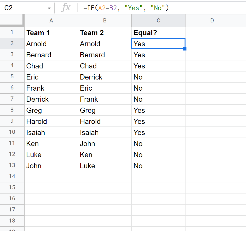

Credit: scales.arabpsychology.com

Identifying Matches And Differences

When working with large sets of data in Google Sheets, it is crucial to be able to compare and analyze multiple columns effectively. The ability to identify matches and differences in your data can provide valuable insights. In this section, we will explore three methods to make this process easier: highlighting exact matches, finding missing values, and detecting unique values.

Highlighting Exact Matches

When you need to identify cells that have the same values in two different columns, highlighting exact matches can be incredibly useful. With conditional formatting in Google Sheets, you can automatically color-code these matching cells to make them stand out.

To highlight exact matches:

Select the two columns you want to compare.
Click on the “Format” tab in the menu bar, then select “Conditional formatting.”
In the “Format rules” drop-down menu, choose “Custom formula is.”
Enter the formula =COUNTIF(range, first_cell) in the text box, replacing range with the range of cells you want to compare and first_cell with the first cell of the range.
Click “Done” to apply the formatting.

Now, any cells with the same values in both columns will be highlighted according to your specified formatting rules, allowing you to easily spot exact matches.

Finding Missing Values

It is also essential to identify any missing values when comparing columns in Google Sheets. Missing values can indicate gaps or inconsistencies in your data, which may require further investigation or corrective measures.

To find missing values:

Select the two columns you want to compare.
Use the =FILTER function combined with the =COUNTIF function to filter out the common values.

This will return only the values that exist in one column but are missing in the other. By examining the resulting data, you can easily identify which values are missing and take appropriate actions.

Detecting Unique Values

Detecting unique values in multiple columns can provide valuable insights into your data. It allows you to identify records that exist only in one column and not in the other, helping you understand the unique characteristics or patterns present in your data.

To detect unique values:

Select the two columns you want to compare.
Use the =FILTER function combined with the =COUNTIF function to filter out the common values.
Apply the =UNIQUE function to the resulting data to extract only the unique values.

You will now have a list of unique values that exist in one column but are not present in the other. This information can be instrumental in identifying outliers or specific data points that require further investigation.

Advanced Techniques

When it comes to advanced techniques in Google Sheets, there are several powerful methods to compare two columns efficiently. These techniques allow for a deeper analysis and insight into your data. In this section, we will explore two key approaches: row-by-row comparisons and combining functions for in-depth analysis. By implementing these advanced techniques, you can easily identify similarities, differences, and patterns in your columns, enabling you to make data-driven decisions with confidence.

Row-by-row Comparisons

Row-by-row comparisons offer a detailed examination of the data in your columns. This technique allows you to perform computations and evaluations on each individual row, providing granular insights. Here are a few methods to conduct row-by-row comparisons:

IF function: The IF function is a versatile tool that allows you to define custom conditions and perform specific actions based on the comparisons made. With the IF function, you can easily compare the values in two columns and generate specific outcomes.
Conditional formatting: Conditional formatting is a fantastic feature in Google Sheets that enables you to highlight cells based on predefined rules. By setting up conditional formatting rules for your two columns, you can visually identify matching or differing values.
VLOOKUP function: The VLOOKUP function is exceptionally handy when comparing two columns. With VLOOKUP, you can search for a value in one column and return the corresponding value from another column. This function is useful for finding matches, differences, and other insights.

Combining Functions For In-depth Analysis

Combining functions takes your analysis to the next level by allowing you to perform complex calculations and evaluations on your data. Here are some powerful functions you can combine to achieve in-depth analysis:

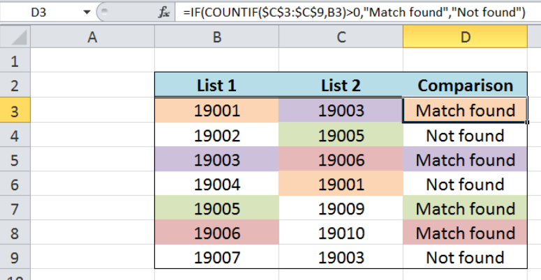
COUNTIF and FILTER: By combining the COUNTIF and FILTER functions, you can compare two columns and return only the common values. This combination allows you to filter out unique or non-matching values, giving you a clear view of the overlapping data.
ARRAYFORMULA and MATCH: The ARRAYFORMULA function, combined with MATCH, can be used to compare two columns and identify matching values. This combination allows you to retrieve the positions or indices of the matching values within your columns.
SUMPRODUCT and EXACT: The SUMPRODUCT function, in tandem with EXACT, is ideal for comparing two columns for exact matches. This combination calculates the sum of logical results returned by the EXACT function, providing you with an accurate count of matching values.

By using these advanced techniques to compare two columns in Google Sheets, you can gain valuable insights into your data. Whether you need a detailed row-by-row analysis or in-depth evaluations using combined functions, these methods empower you to make data-driven decisions efficiently.

Credit: www.got-it.ai

Frequently Asked Questions On Google Sheets Compare Two Columns

How Do I Compare Two Columns In Google Sheets?

To compare two columns in Google Sheets, use conditional formatting to highlight duplicates. Select columns, go to Format, choose Conditional formatting, enter =COUNTIF(range, first_cell) in the formula box, and click Done.

How Do I Compare Two Columns In Google Sheets And Highlight Duplicates?

To compare two columns in Google Sheets and highlight duplicates, select the columns, go to Format, choose Conditional formatting, select Custom formula is, enter the formula =COUNTIF(range, first_cell), and click Done.

How Do You Check If A Value Is In Two Columns In Google Sheets?

To check if a value is in two columns in Google Sheets, use the combination of COUNTIF and FILTER functions. This will compare the two columns and only return the common values. Additionally, you can use VLOOKUP to compare two columns in Google Sheets and highlight duplicates.

How Do I Compare Two Columns In A Spreadsheet?

To compare two columns in a spreadsheet, you can use tools like Google Sheets or Excel. You can start by selecting the two columns you want to compare and use functions like Conditional Formatting or VLOOKUP to highlight duplicates or find missing values.

These tools allow you to easily identify common values or differences between the two columns.

Conclusion

In brief, comparing two columns in Google Sheets is now a breeze with the insightful tips and techniques shared in this blog post. From using conditional formatting to advanced functions like VLOOKUP, you have learned various methods to efficiently compare data and identify duplicates.

Implement these strategies to streamline your data analysis and enhance your productivity in Google Sheets.

Google Sheets Compare Two Columns