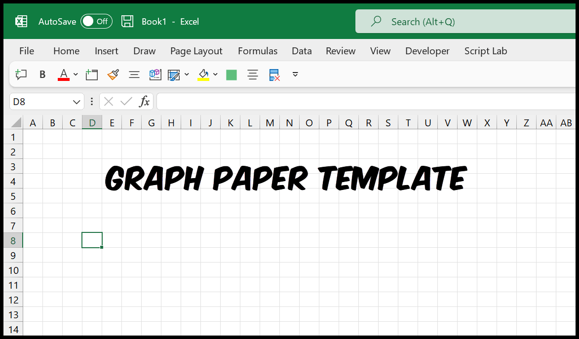
Excel Graph Paper

In Excel, you can create graph paper by changing to “Page Layout” view, selecting all cells, formatting the column width and adjusting the row height. After that, you can return to the normal page view if desired.
This allows you to easily create a grid-like layout for your data. Additionally, you can also make graphs in Excel by clicking anywhere in the data and selecting the type of chart you want to create. From there, you can customize the chart by adding titles, setting axis options, and adding error bars.
With Excel’s versatile features, you can easily create both graph paper and graphs to organize and present your data effectively.
Creating Graph Paper In Excel
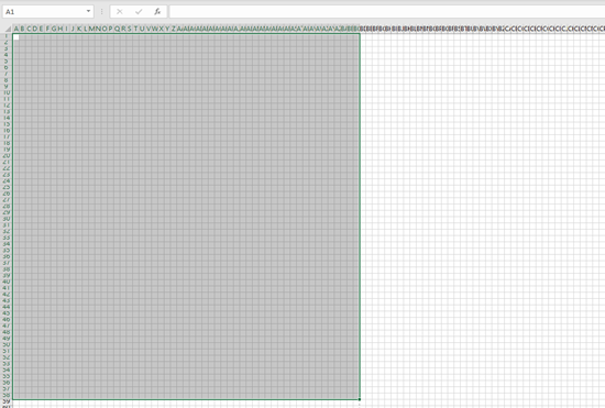
To create graph paper in Excel, switch to “Page Layout” view, open a new empty sheet, select all cells, and format the column width and adjust the row height. You can also return to the ‘Normal’ page view if needed.
With these simple steps, you can easily make graph paper in Excel and use it for various purposes.
Using ‘page Layout’ View
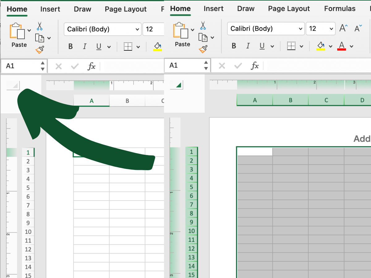
To create graph paper in Excel, start by changing to the ‘Page Layout’ view. Open a new Excel sheet and select all cells by clicking the half triangle button in the upper left corner of the sheet.
Adjusting Column Width And Row Height
Next, format the column width and adjust the row height to your desired dimensions. This step ensures that the graph paper layout is correctly spaced and aligned for your needs.
Making A Chart From Data
To transform the graph paper into a chart, click anywhere on the data you want to visualize. Select ‘Insert > Charts’ and choose the chart type you prefer. Customize the chart options to create a visually appealing representation of your data.
Credit: excelchamps.com
Formatting And Customizing
When it comes to creating visually appealing and informative graphs in Excel, formatting and customizing options play a key role in enhancing the overall look and feel. From adding titles and axis options to exploring various chart design options, Excel makes it easy to customize your graph to suit your specific needs.
Adding Titles And Axis Options
One of the first steps in customizing your Excel graph is adding titles and axis options. By providing clear and concise labels for your graph, you can make it easier for your audience to understand the data presented. To add titles and axis options, follow these simple steps:
- Select your chart by clicking on it.
- Navigate to the Chart Design tab.
- Find the “Chart Title” and “Axis Titles” options.
- Click on the desired title or axis option you want to add.
- Enter the relevant text in the provided field.
- Format the font, size, and style as desired.
- Click “OK” to save your changes.
Exploring Chart Design Options
Excel offers a wide range of chart design options that allow you to customize the appearance of your graph. From changing the colors and styles to adding data labels and trendlines, these design options give you the flexibility to create visually appealing and professional-looking graphs. To explore chart design options, follow these steps:
- Select your chart by clicking on it.
- Navigate to the Chart Design tab.
- Explore the various options available such as chart styles, colors, and effects.
- Select the desired design option to apply it to your graph.
- Modify the design options as needed to achieve the desired visual effect.
- Click “OK” to save your changes.
Printing And Saving
When it comes to using Excel graph paper, printing and saving your customized sheets are essential steps. Whether you need to print a graph paper on a full page or save your customized templates for future use, Excel offers the necessary tools to help you achieve your desired results quickly and easily.
Printing Graph Paper On A Full Page
If you want to print a graph paper on a full page in Excel, follow these simple steps:
- Select the cells containing the graph paper.
- Go to the “Page Layout” view. You can do this by clicking on the “View” tab in the Excel ribbon and selecting “Page Layout”.
- Ensure the selected cells fit the entire page by adjusting the column width and row height. To do this, select the cells and click on the half triangle button in the upper left corner of the sheet. Then, choose the desired column width and row height.
- Once you are satisfied with the layout, return to the “Normal” page view by clicking on the “View” tab and selecting “Normal”.
- Finally, you can print your graph paper by going to the “File” tab, selecting “Print”, and adjusting the print settings according to your preferences. Remember to choose the correct printer and paper size before printing.
Saving Customized Graph Paper
Excel allows you to save your customized graph paper templates for future use. To save your graph paper, follow these steps:
- Select the cells containing the customized graph paper.
- Go to the “File” tab and select “Save As”.
- Choose the desired location on your computer where you want to save the file.
- Enter a name for the file and select the file format you prefer, such as Excel Workbook (.xlsx).
- Click on “Save” to save the file.
By following these steps, you can easily print your graph paper on a full page or save your customized templates in Excel. This feature is incredibly useful when working on different projects or needing to share your graph paper with others. Start using Excel today and enjoy the convenience it offers for creating and managing graph paper!
Credit: www.automateexcel.com
Additional Resources
To create Excel graph paper, change to ‘Page Layout’ view, open a new empty Excel sheet, select all cells, and format the column width and adjust the row height. Then, return to ‘Normal’ page view. Additionally, you can make a chart by clicking anywhere in the data and selecting Insert > Charts > the chart type you want.
Graph Paper Templates And Related Content
Explore various graph paper templates and related content for your Excel projects:
- Grid Template
- Isometric Graph Paper
- Polar Graph Paper
Related Content
Discover more about using Excel for graphing and data visualization:
- Creating Dynamic Charts in Excel
- Data Analysis with Excel
- Advanced Chart Formatting Techniques
Credit: www.knittinghousesquare.com
Frequently Asked Questions On Excel Graph Paper
Can I Make Graph Paper In Excel?
Yes, you can create graph paper in Excel by adjusting column width, row height, and layout settings.
How Do I Make An Excel Graph?
To make an Excel graph, follow these steps: 1. Click anywhere in the data you want to graph. 2. Select Insert > Charts and choose the desired chart type. 3. Customize your graph using the options provided. 4. Click “OK” to create the graph.
Source: Microsoft Support.
How Do I Graph A Worksheet In Excel?
To graph a worksheet in Excel, follow these steps: 1. Change to “Page Layout” view. 2. Open a new empty Excel sheet. 3. Select all cells and click on the half triangle button in the upper left corner of the sheet.
4. Format the column width and adjust the row height. 5. Return to ‘Normal’ page view (optional).
How Do You Make An Excel Graph Its Own Sheet?
To make an Excel graph its own sheet, go to Chart Design tab, click Move Chart, select New sheet in the dialog box.
Conclusion
Creating graph paper in Excel is a simple process with great convenience. By following the steps mentioned, you can easily customize and print your graph paper in Excel. Enhance your data visualization and organizational skills with this handy Excel feature.
Start graphing today!